27 KiB
_model: slides
title: CSCI 577 - Data Mining
body:
Political Polarization
CSCI 577
Matt Jensen
May 18, 2023
==
Outline
- Hypothesis
- Sources
- Data Workup
- Experiments
- Remaining Work
- Questions
===
Hypothesis
==
Hypothesis
Political polarization is rising, and news articles are a proxy measure.
==
Why might we expect this?
Mostly anecdotal experience.
Evidence is mixed in the literature 1,2,3.
Our goal is whether, not why.
Note:
Proliferation of media choices lowered the share of less interested, less partisan voters and thereby made elections more partisan. But evidence for a causal link between more partisan messages and changing attitudes or behaviors is mixed at best. Measurement problems hold back research on partisan selec- tive exposure and its consequences. Ideologically one-sided news exposure may be largely confined to a small, but highly involved and influential, seg- ment of the population. There is no firm evidence that partisan media are making ordinary Americans more partisan.
==
Sub-hypothesis
- The polarization is not evenly distributed across publishers.
- The polarization is not evenly distributed across political specturm.
- The polarization increases near elections.
==
Sub-sub-hypothesis
- Similarly polarized publishers link to each other.
- 'Mainstream' media uses more neutral titles.
- Highly polarized publications don't last as long.
Note:
- Publication longivity is not covered currently.
- Mainstream media dominates the dataset.
===
Data Sources
==
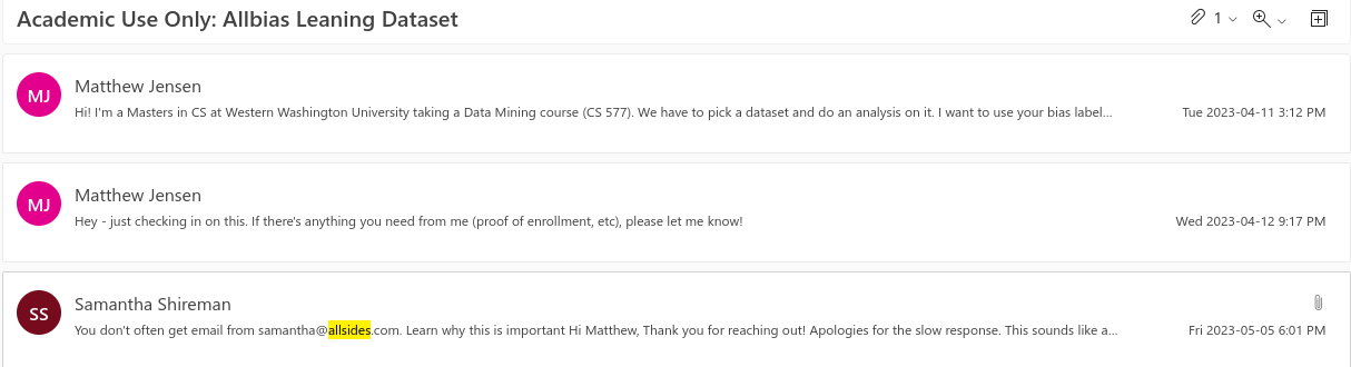
Data Sources
- Memeorandum: stories
- AllSides: bias
- HuggingFace: sentiment
- ChatGPT: election dates
Note:
Let's get a handle on the shape of the data.
- sources
- size
- features
===
Memeorandum
==
==
Memeorandum
- News aggregation site.
- Was really famous before Google News.
- Still aggregates sites today.
==
Memeorandum
- I still use it.
- I like to read titles.
- Publishers block bots.
- Simple html to parse.
- Headlines from 2006 forward.
- Automated, not editorialized.
Note:
- It limits doom scrolling.
===
AllSides
==
==
AllSides
- Rates publications as left, center or right.
- Ratings combine:
- blind bias surveys.
- editorial reviews.
- third party research.
- community voting.
Note: Originally scraped website, but direct access eventually.
==
AllSides
- One of the only bias apis.
- Ordinal ratings [-2: very left, 2: very right].
- Covers 1400 publishers + some blog and authors.
- Easy format and semi-complete data.
===
HuggingFace
==
==
HuggingFace
- Deep learning library.
- Lots of pretrained models.
- Easy, off the shelf word/sentence embeddings and text classification models.
==
HuggingFace
- Language models are HOT.
- Literally 5 lines of python.
- The dataset needed more features.
- Testing different model performance was easy.
- Lots of pretrained classification tasks.
===
Data Collection
==
Data Collection
Stories
day = timedelta(days=1)
cur = date(2005, 10, 1)
end = date.today()
while cur <= end:
    cur = cur + day
    save_as = output_dir / f"{cur.strftime('%y-%m-%d')}.html"
    url = f"https://www.memeorandum.com/{cur.strftime('%y%m%d')}/h2000"
    r = requests.get(url)
    with open(save_as, 'w') as f:
        f.write(r.text)
Note:
grab every page from 2005 forward.
later: parse it into csv/database.
==
Data Collection
Bias hard
...
bias_html = DATA_DIR / 'allsides.html'
parser = etree.HTMLParser()
tree = etree.parse(str(bias_html), parser)
root = tree.getroot()
rows = root.xpath('//table[contains(@class,"views-table")]/tbody/tr')

ratings = []
for row in rows:
    rating = dict()
    ...
Note:
grab entire index
later parse it into csv/database
==
Data Collection
Bias easy
Note:
json format, including authors and blogs.
==
Data Collection
Embeddings
# table = ...
tokenizer = AutoTokenizer.from_pretrained("roberta-base")
model = AutoModel.from_pretrained("roberta-base")

for chunk in table:
    tokens = tokenizer(chunk, add_special_tokens = True, truncation = True, padding = "max_length", max_length=92, return_attention_mask = True, return_tensors = "pt")
    outputs = model(**tokens)
    embeddings = outputs.last_hidden_state.detach().numpy()
    ...
Note:
for every title, tokenize then embed.
hidden state is last linear layer before training tasks.
==
Data Collection
Classification Embeddings
...
outputs = model(**tokens)[0].detach().numpy()
scores = 1 / (1 + np.exp(-outputs))  # Sigmoid
class_ids = np.argmax(scores, axis=1)
for i, class_id in enumerate(class_ids):
    results.append({"story_id": ids[i], "label" : model.config.id2label[class_id]})
...
Note:
for every title, tokenize, classify.
~ 1 hour
===
Data Structures
Stories
Note:
Great, we have the data, now what does it look like?
==
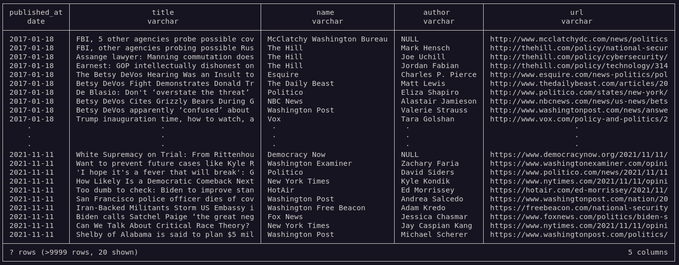
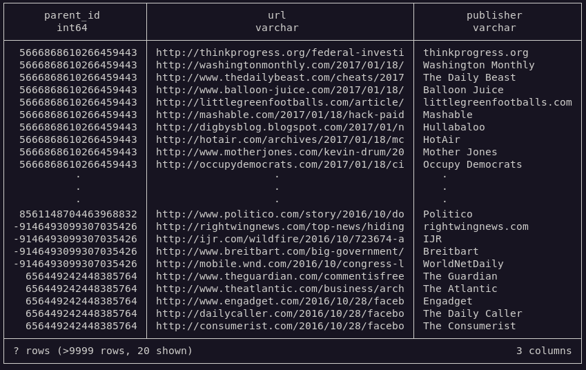
Data Structures
Stories
- Top level stories.
- title, author, publisher, url, date.
- Related discussion.
- publisher, url.
- uses 'parent' story as a source.
- Story stream changes constantly (dedup. required).
==
Data Structures
Stories
==
Data Structures
Stories
==
Data Structures
Stories
| metric | value |
|---|---|
| total stories | 299714 |
| total related | 960111 |
| publishers | 7031 |
| authors | 34346 |
| max year | 2023 |
| min year | 2005 |
| top level domains | 7063 |
==
Data Selection
Stories
- Clip the first and last full year of stories.
- Remove duplicate stories (big stories span multiple days).
- Convert urls to tld to link to publishers.
Note:
tld: top level domain.
==
Data Selection
Publishers
- Combine subdomains of stories.
- blog.washingtonpost.com and washingtonpost.com are considered the same publisher.
- This could be bad. For example: opinion.wsj.com != wsj.com.
- Find common name of publisher.
Note:
Sometime authors are the publisher name.
==
Data Selection
Related
- Select only stories with publishers whose story had been a 'parent' ('original publishers').
- Eliminates small blogs and non-original news.
- Eliminate publishers without links to original publishers.
- Eliminate silo'ed publications.
- Link matrix is square and low'ish dimensional.
Note:
Going to build a data structure of the related links, so I have to be judicious about which ones to include.
==
Data Selection
Post Process
| metric | value |
|---|---|
| total stories | 251553 |
| total related | 815183 |
| publishers | 223 |
| authors | 23809 |
| max year | 2022 |
| min year | 2006 |
| top level domains | 234 |
Note:
much less publishers, but count(stories) about the same - main stream represent.
==
Descriptive Stats
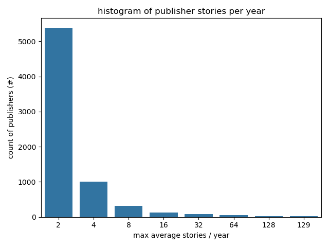
Stories Per Publisher
Note:
Power law in effect.
==
Descriptive Stats
Top Publishers
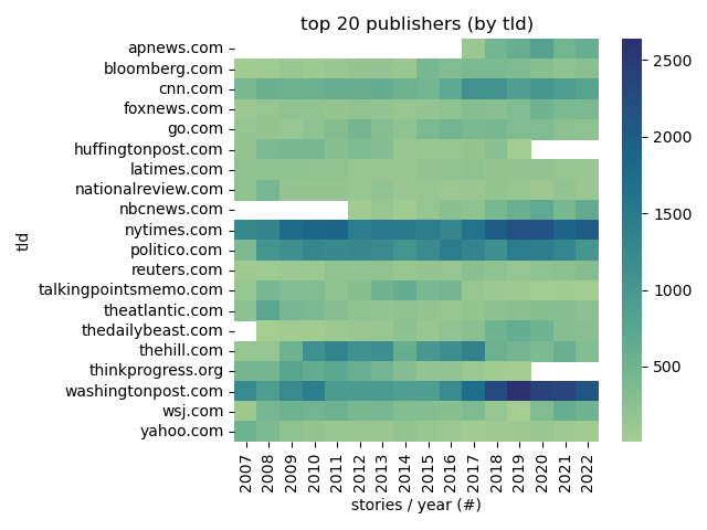
Note:
Some publishers come and go.
Some publishers change their domains.
==
Descriptive Stats
Articles Per Year
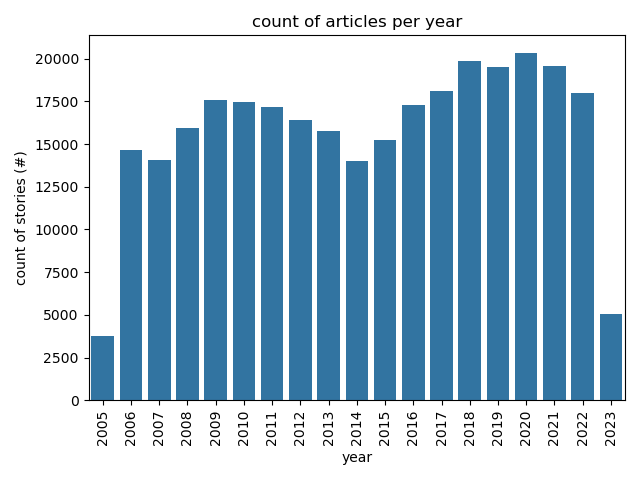
Note:
Shape of total articles per year dominates some of the analysis.
==
Descriptive Stats
Common TLDs
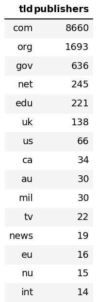
Note:
just for funs.
Lots of IP addresses and spammy looking ones.
===
Data Structures
Bias
==
Data Structures
Bias
- Per publisher.
- name,
- label/ordinal value.
- agree/disagree vote by community.
- Name could be semi-automatically joined to stories.
==
Data Structures
Bias
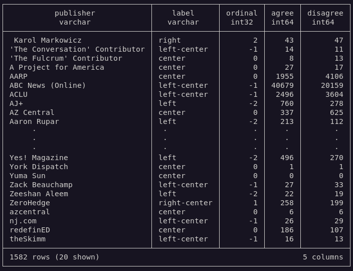
Note:
Later, media type and explicit ordinal values were added via api access.
==
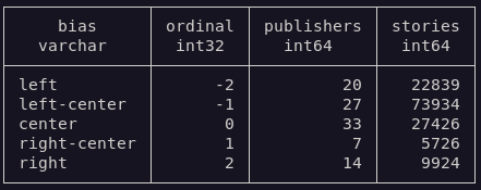
Data Selection
Bias
- Keep all ratings.
- Join datasets on publisher name.
- Started with 'jaro winkler similarity' then manually from there (look up Named Entity Recognition).
- Use numeric values.
- [left: -2, left-center: -1, ...].
- Possibly scale ordinal based on agree/disagree ratio.
Note:
Lots of agrees on the ends of the spectrum implies their very left or very right.
Lots of agrees in the middle implies very neutral?
==
Data
Bias
==
Data
Bias
Note:
much smaller dataset.
TODO: manually add more joins to story source.
===
Data Structures
Embeddings
==
Data Structures
Embeddings
- Per story title.
- sentence embedding (n, 384) - BERT.
- sentiment classification (n, 1) - RoBERTa base.
- emotional classification (n, 1) - RoBERTa Go-Emotions.
- ~ 1 hour of inference time to map story titles and descriptions.
Note:
RoBERTa - pretrained with the Masked language modeling (MLM) objective. Taking a sentence, the model randomly masks 15% of the words in the input then run the entire masked sentence through the model and has to predict the masked words.
SST - Stanford Sentiment Treebank: 11,855 single sentences extracted from movie reviews, annotated by 3 human judges.
==
Data Selection
Embeddings
- Word embeddings were too complicated.
- Kept argmax of classification prediction ([0.82, 0.18] -> LABEL_0).
- For publisher based analysis, averaged sentence embeddings for all stories.
==
Data
Embeddings
| label | stories | publishers |
|---|---|---|
| positive | 87830 | 223 |
| negative | 163723 | 223 |
Note:
There was a model with a neutral label as well, but I opted out.
==
Data
Embeddings
| label | stories | publishers |
|---|---|---|
| neutral | 124257 | 223 |
| anger | 34124 | 223 |
| fear | 36756 | 223 |
| sadness | 27449 | 223 |
| disgust | 17939 | 222 |
| surprise | 5710 | 216 |
| joy | 5318 | 214 |
===
Experiments
==
Experiments
- clustering on link similarity.
- classification on link similarity.
- classification on sentence embedding.
- classification on sentiment analysis.
- regression on emotional classification over time and publication.
Note:
5 main experiments.
Lots of tinkering and 'agile development'.
Use source control.
===
Experiment 1
clustering on link similarity.
==
Experiment 1
Setup
- Create one-hot encoding of links between publishers.
- Cluster the encoding.
- Expect similar publications in same cluster.
- Use PCA to visualize clusters.
Note: Principle Component Analysis:
- a statistical technique for reducing the dimensionality of a dataset.
- linear transformation into a new coordinate system where (most of) the variation data can be described with fewer dimensions than the initial data.
- I use it alot to map from high dimensional space (links adj. and embeddings) to lower, most significant space.
==
Experiment 1
Encoding schemes
==
Experiment 1
One-hot Encoding
| publisher | nytimes | wsj | newsweek | ... |
|---|---|---|---|---|
| nytimes | 1 | 1 | 1 | ... |
| wsj | 1 | 1 | 0 | ... |
| newsweek | 0 | 0 | 1 | ... |
| ... | ... | ... | ... | ... |
==
Experiment 1
n-Hot Encoding
| publisher | nytimes | wsj | newsweek | ... |
|---|---|---|---|---|
| nytimes | 11 | 1 | 141 | ... |
| wsj | 1 | 31 | 0 | ... |
| newsweek | 0 | 0 | 1 | ... |
| ... | ... | ... | ... | ... |
==
Experiment 1
Normalized n-Hot Encoding
| publisher | nytimes | wsj | newsweek | ... |
|---|---|---|---|---|
| nytimes | 0 | 0.4 | 0.2 | ... |
| wsj | 0.2 | 0 | 0.4 | ... |
| newsweek | 0.0 | 0.0 | 0.0 | ... |
| ... | ... | ... | ... | ... |
==
Experiment 1
Elbow criterion
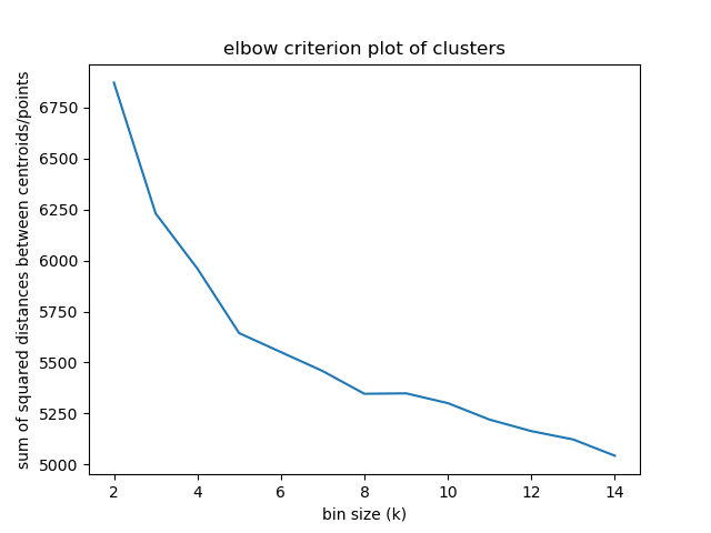
Note:
The elbow method looks at the percentage of explained variance as a function of the number of clusters:
One should choose a number of clusters so that adding another cluster doesn't give much better modeling of the data.
Percentage of variance explained is the ratio of the between-group variance to the total variance
sklearn eliminated 2 cluster groups??
==
Experiment 1
Comparing encoding schemes
Note:
They all have good clusters.
==
Experiment 1
Link Magnitude
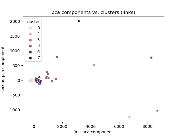
Note:
link frequency dominates one component.
more interested in bias between publishers, not difference between mainstream and outliers.
==
Experiment 1
Normalized
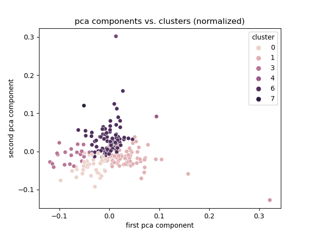
Note:
a few outliers still, but better.
==
Experiment 1
One-Hot
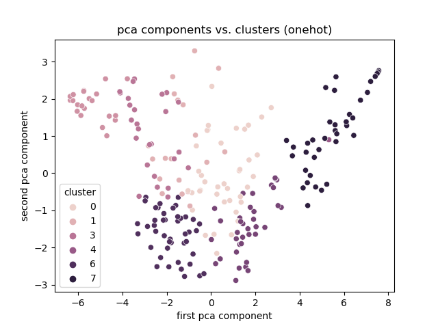
Note:
really dispursed
==
Experiment 1
Discussion
- One-hot seems to reflect the right features.
- Found clusters, but meaning is arbitrary.
- map to PCA results nicely.
- Limitation: need the link encoding to cluster.
- Smaller publishers might not link very much.
- TODO: Association Rule Mining.
- 'Basket of goods' analysis to group publishers.
===
Experiment 2
classification on link similarity.
==
Experiment 2
Setup
- Create features:
- Publisher frequency.
- Reuse link encodings.
- Create classes:
- Join bias classifications.
- Train classifier.
Note:
==
Experiment 2
Descriptive stats
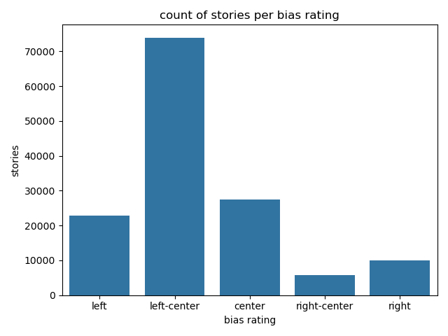
| metric | value |
|---|---|
| publishers | 1582 |
| labels | 6 |
| left | 482 |
| center | 711 |
| right | 369 |
| agree range | [0.0-1.0] |
Note:
rehash of what bias data is available.
==
Experiment 2
Results
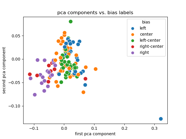
Note:
pca maps to bias labels well, left on one end, right on the other.
if you squint.
==
Experiment 2
Results
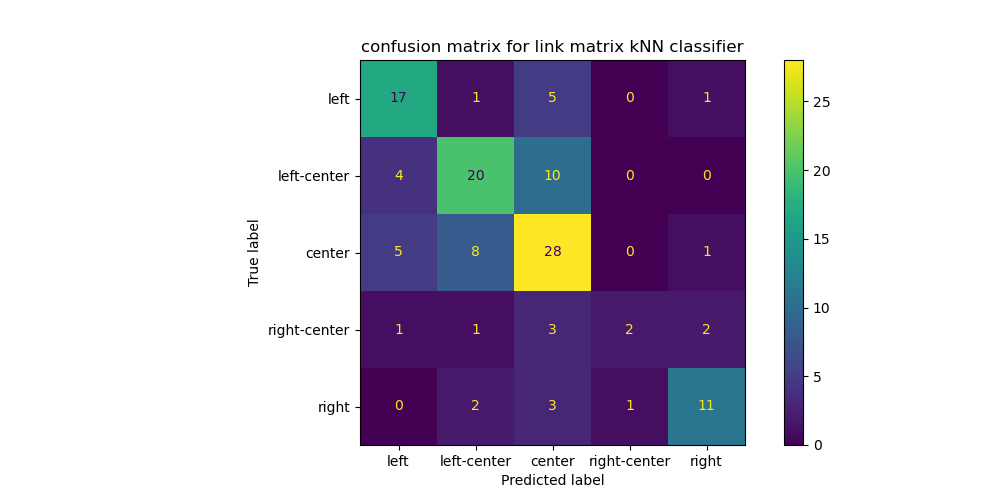
Note:
hot diagonal is good.
all data.
train test split only had 20 or so samples in it?
overlap between link choices and bias ratings is slim.
==
Experiment 2
Discussion
- Link encodings (and their PCA) are useful.
- Labels are (sort of) separated and clustered.
- Creating them for smaller publishers is trivial.
- Hot diagonal confusion matrix is good.
- Need to link more publisher data to get good test data.
Note:
==
Experiment 2
Limitations
- Dependent on accurate rating.
- Ordinal ratings weren't available.
- Dependent on accurate joining across datasets.
- Entire publication is rated, not authors.
- Don't know what to do with community rating.
===
Experiment 3
classification on sentence embedding.
==
Experiment 3
Setup
- Generate sentence embedding for each title.
- Rerun PCA analysis on title embeddings.
- Use kNN classifier to map embedding features to bias rating.
==
Experiment 3
Embeddings Primer
==
Experiment 3
Embedding Steps
- Extract titles.
- Tokenize titles.
- Pick pretrained language model.
- Generate embeddings from tokens using model.
==
Experiment 3
Tokens
The sentence:
"Spain, Land of 10 P.M. Dinners, Asks if It's Time to Reset Clock"
Tokenizes to:
['[CLS]', 'spain', ',', 'land', 'of', '10', 'p', '.', 'm', '.',
    'dinners', ',', 'asks', 'if', 'it', "'", 's', 'time', 'to',
    'reset', 'clock', '[SEP]']
Note: [CLS] is unique to BERT models and stands for classification.
==
Experiment 3
Tokens
The sentence:
"NPR/PBS NewsHour/Marist Poll Results and Analysis"
Tokenizes to:
['[CLS]', 'npr', '/', 'pbs', 'news', '##ho', '##ur', '/', 'maris',
    '##t', 'poll', 'results', 'and', 'analysis', '[SEP]', '[PAD]',
    '[PAD]', '[PAD]', '[PAD]', '[PAD]', '[PAD]', '[PAD]']
Note: The padding is there to make all tokenized vectors equal length.
The tokenizer also outputs a mask vector that the language model uses to ignore the padding.
==
Experiment 3
Embeddings
- Using a BERT (Bidirectional Encoder Representations from Transformers) based model.
- Input: tokens.
- Output: dense vectors representing 'semantic meaning' of tokens.
==
Experiment 3
Embeddings
The tokens:
['[CLS]', 'npr', '/', 'pbs', 'news', '##ho', '##ur', '/', 'maris',
    '##t', 'poll', 'results', 'and', 'analysis', '[SEP]', '[PAD]',
    '[PAD]', '[PAD]', '[PAD]', '[PAD]', '[PAD]', '[PAD]']
Embeds to a vector (1, 384):
array([[ 0.12444635, -0.05962477, -0.00127911, ...,  0.13943022,
        -0.2552534 , -0.00238779],
       [ 0.01535596, -0.05933844, -0.0099495 , ...,  0.48110735,
         0.1370568 ,  0.3285091 ],
       [ 0.2831368 , -0.4200529 ,  0.10879617, ...,  0.15663117,
        -0.29782432,  0.4289513 ],
       ...,
Note:
attention masks allow the model to ignore padding so all vectors are same length.
embedding space has semantic meaning.
can do vector math on them:
king - man = monarch
monarch + dance = happy?
==
Experiment 3
Results
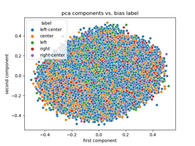
Note:
pca on the sentence embeddings of the titles.
not a lot of information in PCA this time.
==
Experiment 3
Results
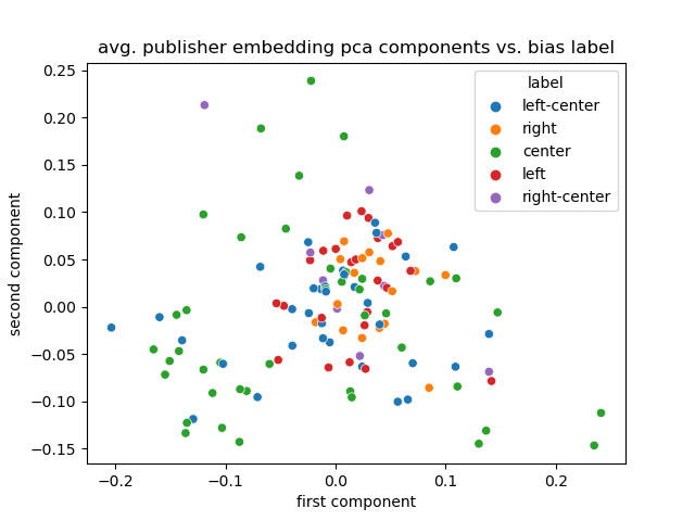
Note:
What about average publisher embedding?
centers are pushed outside?
sorry about the color pallet.
==
Experiment 3
Results
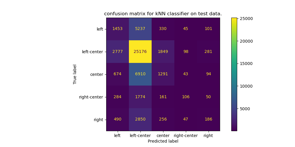
Note: Trained a kNN from sklearn.
Set aside 20% of the data as a test set.
Once trained, compared the predictions with the true on the test set.
not bad.
==
Experiment 3
Discussion
- Embedding space is hard to condense with PCA.
- Maybe the classifier is learning to guess 'left-ish'?
- Does DL work better on sparse inputs?
===
Experiment 4
classification on sentiment analysis.
==
Experiment 4
Setup
- Use pretrained language classifier.
- Previously: Mapped twitter posts to tokens, to embedding, to ['positive', 'negative'] labels.
- Predict: rate of neutral titles decreasing over time.
==
Experiment 4
Results
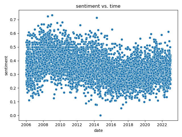
Note:
maybe there's something there.
less positive after 2008?
low around 2016?
increase around 202?
overall still lower.
==
Experiment 4
Results
Note:
right has not a lot of data.
all trend down over time.
people loved Obama at the beginning.
==
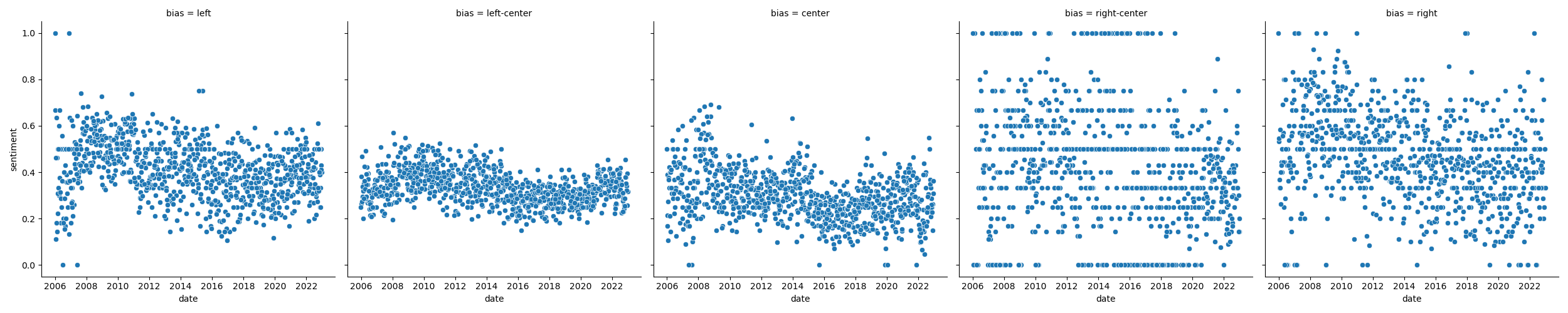
Experiment 4
Results
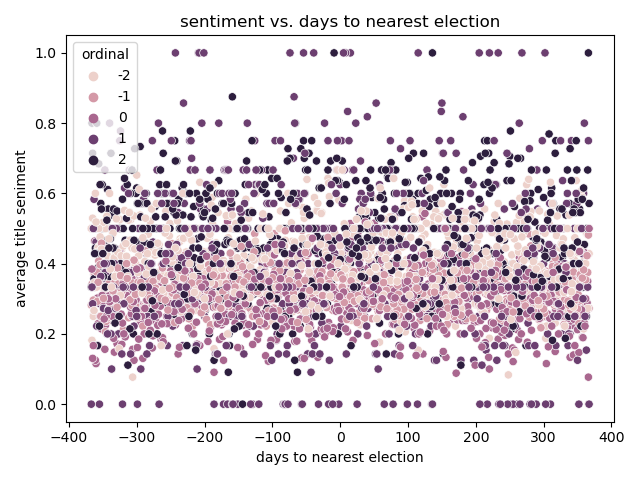
Note:
assumption: national elections drive news sentiment.
expected a taller band in the middle then the edges.
==
Experiment 4
Discussion
- Bump post Obama election for left and center.
- Dip pre Trump election for left and center.
- Right is all over the place - not enough data?
- Recency of election not a clear factor.
===
Experiment 5
regression on title emotional expression.
==
Experiment 5
Setup
- Use pretrained language classifier.
- Previously: Mapped reddit posts to tokens, to embedding, to emotion labels.
- Predict: rate of neutral titles decreasing over time.
- Classify:
- features: emotional labels
- labels: bias
==
Experiment 5
Results
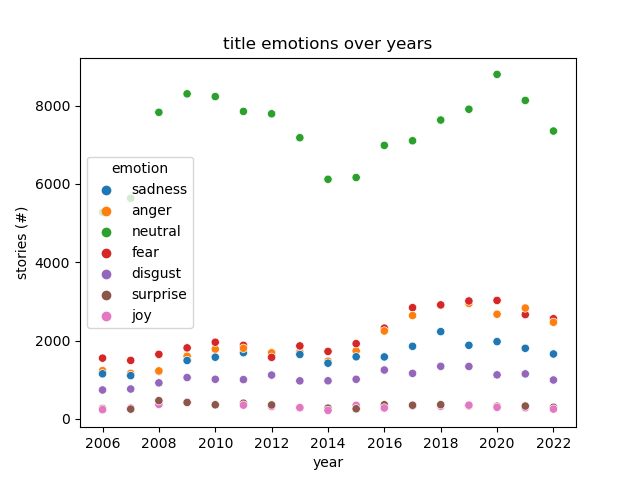
Note:
neutrality between Obama and Trump
emotional titles all increased - shape of the underlying data.
TODO: normalize relative expression.
==
Experiment 5
Results
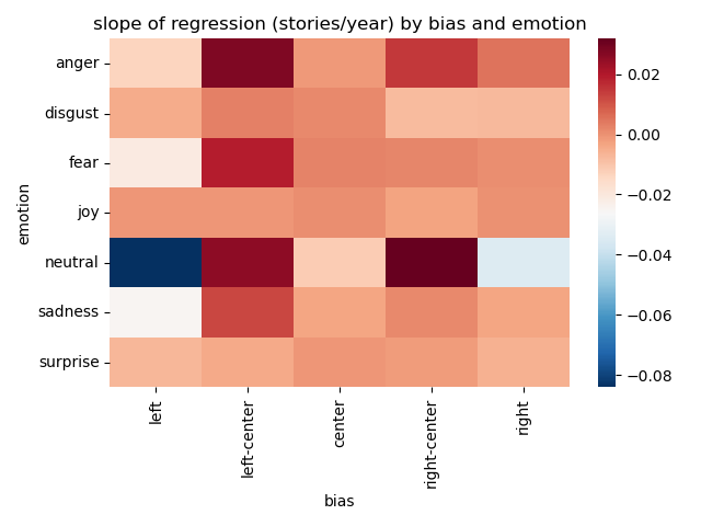
Note:
left and right got less neutral over time.
==
Experiment 5
Discussion
- Neutral story titles dominate the dataset.
- Increase in stories published might explain most of the trend.
- Far-right and far-left both became less neutral.
- Left-Center and right-center became more emotional, but also neutral.
- Not a lot of movement overall.
===
Conclusion
==
Hypothesis
- The polarization is not evenly distributed across publishers. unproven
- The polarization is not evenly distributed across political specturm. unproven
- The polarization increases near elections. false
- Similarly polarized publishers link to each other. sorta
- 'Mainstream' media uses more neutral titles. true
- Highly polarized publications don't last as long. untested
==
Conclusion
- Article titles do not have a lot of predictive power.
- Mainstream, neutral publications dominate the dataset.
- Link frequency, sentence embeddings, and sentiments are useful features.
- A few questions remain.
Note:
Experiment 6 (TODO)
- Have a lot of features now.
- Link PCA components.
- Embedding PCA components.
- Sentiment.
- Emotion.
- Can we predict with all of them: Bias.
limitations
- Many different authors under the same publisher.
- Publishers use syndication.
- Bias ratings are biased and not linked automaticall.
- National news is generally designed to be neutral sounding.
- End user: Is that useful? Where will I get all that at inference time?
==
Questions
==
References
[1]: Stewart, A.J. et al. 2020. Polarization under rising inequality and economic decline. Science Advances. 6, 50 (Dec. 2020), eabd4201. DOI:https://doi.org/10.1126/sciadv.abd4201.
Note: